-
2.1
Auto-Pipe: The Bigger Picture
2.2 Sample Application Mapping
2.3 X-Sim Details
- 3.1 The Real World System
3.2 The Analytic Model
3.3 The Simulation Program 4 Verification and Validation Theory
-
4.1 Conceptual Model Validation: the System-Model
Relationship
4.2 Model Verification: the Model-Program Relationship
4.3 Operational Validation: the System-Program Relationship
- 5.1 Conceptual Model Validation Results
5.2 Model Verification Results
5.3 Operational Validation Results
5.4 Summary
7 References
8 Acronyms
1 Introduction
For any simulation to have credibility, it is necessary to verify and validate the results of the simulation. This allows target users to have sufficient confidence that results generated by a simulation run reflect real world operation to a large degree. This paper focuses on the verification and validation of X-Sim [Gayen05], a simulator built for the Auto-Pipe [Tyson06] system. The Auto-Pipe system is a comprehensive package focused on facilitating the deployment and optimization of scientific applications on heterogeneous resources. Heterogeneous resources are defined to include physical resources such as general purpose processors (GPPs), field programmable gate arrays (FPGAs), graphical processor units (GPUs), etc., and their physical interconnects such as ethernet, PCI, etc. X-Sim is a vital component of the system, as it allows correctness checking and performance prediction before actual deployment. Performance predictions can be used to create more optimal mappings of the application to a given resource set. This paper uses a single example to illustrate application deployment in the Auto-Pipe system, as well as simulation of the deployed application. Verification and validation is performed on the sample application, while illustrating how similar techniques can be applied to any application deployed in the Auto-Pipe system.2 X-Sim
2.1 Auto-Pipe: the Bigger Picture
X-Sim is a simulator built for the Auto-Pipe system [Gayen06]. Auto-Pipe is a performance-oriented development environment for heterogeneous systems. It concentrates on streaming applications placed on pipelined architectures. In this system, applications are expressed in the X Language [Tyson05] as dataflow graphs. In these graphs, individual computational tasks called blocks are connected with interconnects called edges indicating the type and flow of data between blocks. The actual implementations of the blocks are written in various languages for any subset of the available platforms (e.g., C for general-purpose processors, HDL for FPGAs, assembly for network processors and DSPs). Applications may be mapped onto arbitrary sets of mixed physical resources. Such resources may be a combination of general-purpose processors (e.g., x86, PowerPC, ARM), chip multiprocessors (e.g., Intel IXP network processor, multi-core x86 processors), and reconfigurable hardware devices (e.g., FPGAs).
2.2 Sample Application Mapping
Throughout this paper, the simple example application mapping problem shown in Figure 1 will be used for illustrative purposes.
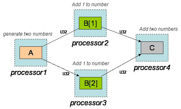
Figure 1 : A sample application in the Auto-Pipe System
The example consists of four blocks mapped to four processors. This single mapping will be used to illustrate the various simulation verification and validation techniques presented in this paper. Block A, mapped to a processor processor1, is a generator block that creates ten pairs of 32-bit unsigned numbers. These unsigned32's are streamed in parallel through a pair of add1 blocks, B[1] and B[2]. In addition to adding one to the unsigned32 passing through, each B block runs long loops that increment a dummy temp value n number of times, where n is a random variable uniformly distributed between 200,000 and 250,000. The random number generator used is the GNU C library's rand() function. The two B blocks are mapped to separate processors, processor2 and processor3. Their outputs are streamed into a summation block, C, mapped to processor processor4. All of the processors used in this example are identical Pentium 4 machines, with speed 3.4Ghz and memory 512MB.
2.3 X-Sim Details
Within the Auto-Pipe system, X-Sim [Gayen06] provides functional simulation to determine application correctness, and performance simulation to profile individual components of the application. The results of performance simulation may then be used to improve the performance either manually or automatically using an optimization application currently under development, X-Opt. X-Sim provides an environment in which multiple simulators are seamlessly combined to simulate X Language applications mapped to heterogeneous devices. The X-Sim infrastructure is open-ended to allow support for a range of simulators, from low-level discrete-event and cycle-accurate simulators to rough estimates from emulators and native execution. X-Sim records timestamps for each block. Whenever data enters or exits a block, a copy of the data is stored and a timestamp is recorded. By the end of the simulation run, a complete trace of all data and timestamps is generated. The data traces are useful in correctness checking, and the timestamps are useful in understanding system performance. The traces represent a comprehensive set of data gathered from the simulation.
3 Simulation Theory
For any simulation project, there are three main entities: the real world system, the analytic model, and the simulation program [Sargent 04]. Briefly, the real world system is the system we want to study, the analytic model is the analytic representation of the system, and the simulation program is the computer program that is used to simulate the system. The rest of this section describes how the example application fits into this view of simulation.
3.1 The Real World System
The real world system consists of all the real world elements we are
interested in studying. In the Auto-Pipe system, the system consists of the
application that we want to optimize, the physical computational resources such
as computers and specialized hardware, and the communication interconnects that
connect the
computational resources. In our example, the application consists of the five
code blocks introduced in the previous section. The computational resources
consist of the four pentiums described before, and the interconnect resources
consist of the ethernet links between the Pentiums. All these components make up
the system that we want to study, run, and optimize.
3.2 The Analytic Model
The analytic model is the analytic representation of the system. It includes representations of each of the real world system components, and has equations and guiding heuristics that characterize the behaviour of each component. In the Auto-Pipe system, the entire application is treated as an M/M/1 queueing network. It is assumed that each node (computational resource or interconnect resource) has exponentially distributed inter-arrival and service times.
3.3 The Simulation Program
The simulation program is written by a programmer to simulate the analytic model. X-Sim is written in C++, as is the rest of the Auto-Pipe system. It is written in classic object oriented format, with classes built for individual modules within the program.
4 Verification and Validation Theory
4.1 Conceptual Model Validation: the System-Model Relationship
The queuing network model assumes that each node has exponentially distributed inter-arrival and service times. These assumptions need to be validated statistically to conceptually validate the model [Balci 95]. Each of these distributions' characteristics parameters are set according to results obtained from simulation runs. In accepting or rejecting the analytic model, two types of errors are possible: Type I errors and Type II errors. Type I error is an error where a valid model is rejected, and Type II error is an error where an invalid model is accepted. Type II errors are considered particularly bad, and must be minimized. The process of validating that the analytic model closely approximates the behavior of the real world is called conceptual model validation.
4.2 Model Verification: the Model-Program Relationship
Model verification is the process of verifying that the program runs correctly, in a manner that reflects the analytic model. Techniques that can be used for model verification include walk-throughs, correctness proofs, and sanity checks. For the example application, walk throughs were done to verify that data moved through the simulation modules as expected for a few test cases. A rudimentary sanity check was done by confirming that block output times occured chronologically after block input times. It is hard to quantify program correctness, and a technique that can help in verification is an animation . A tool that shows the movement of data through the queue network model is currently under construction. Once it is completed, it can help the programmer quickly locate suspicious behaviour which might indicate the presence of programming errors.
4.3 Operational Validation: the System-Program Relationship
A major part of providing credibility to X-Sim's results is proving operational validity [Kleijnen 95]. Operational validation is defined as the process of confirming that simulation results closely approximate real world results. X-Sim runs are able to generate comprehensive timestamps for each data transaction that happens on any device. Real world system runs, on the other hand, only generate means for the service time for each device. The difference occurs because simulators can gather data in a more non-obtrusive manner, affecting block performance minimally. Real world executions, on the other hand, suffer a higher performance penalty if timestamps for each and every data transaction are recorded. To minimize the effect on performance, only means can currently be recorded from real world system runs. Additional work will be done in the future to enable timestamps to be gathered for the real world system runs as well. This data can be used in operational validation if one keeps in mind the fact that this more detailed trace capture has more significant effects on system performance. A comprehensive set of experiments were run to analyze conceptual model validation (how closely the analytic model approximates the real system) and operation validation (how closely simulation results match real system results).
5 Experimental Results and Analysis
Several experiments were run to verify and validate the relationships between the system, the model, and the program.
5.1 Conceptual Model Validation Results
A single simulation run was done to check the underlying assumptions of the conceptual model, that the inter-arrival times and service times of the nodes are exponentially distributed. The example application discussed previously was simulated and timestamps captured for every data transaction. Note that in a single simulation run, 10000 jobs arrive and get serviced at every node in the queue network. To check the assumptions underlying the queuing model, the timestamps at the exit port of block B[1] were taken and processed to generate inter-arrival times. The Quantile-Quantile plot (hereafter referred to as Q-Q plot) is plotted below.
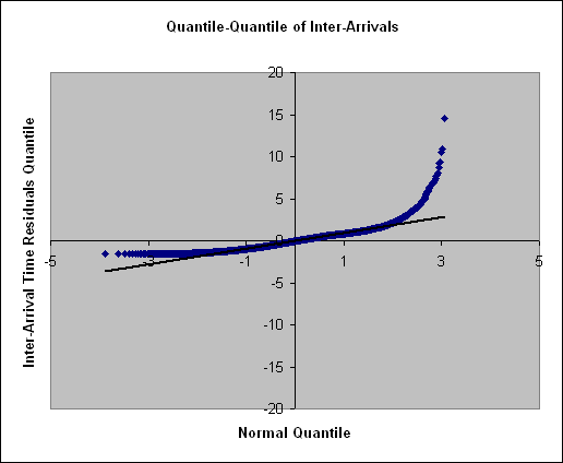
Figure 2: Q-Q Plot of Inter-Arrival Times for Block B[1]
The figure clearly shows that the arrival times are exponentially distributed. Another assumption that needs to be tested is to see if the distribution of the service times is also exponentially distributed. To test this, a Q-Q plot of the service times for block B[1] is shown below in Figure 3.
.
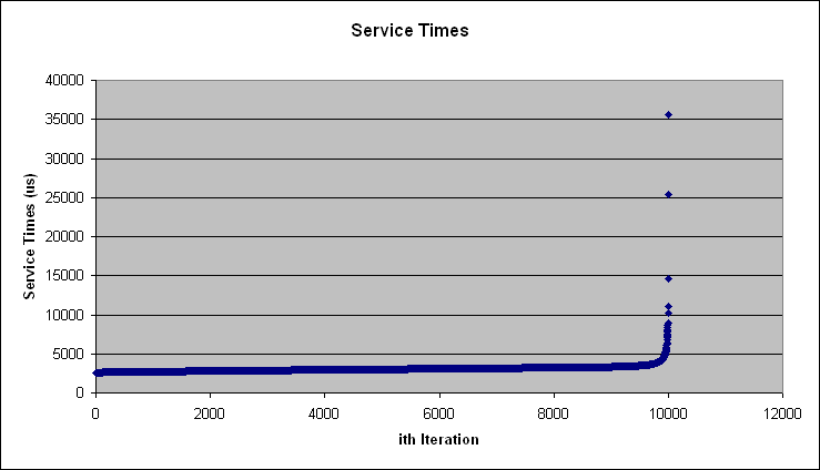
Figure 3: Q-Q plot of Service Times for Block B[1]
This figure shows that at least 5 data points are extreme outliers. Excluding the 10 top outliers produces Figure 4, shown below. This figure is a bit clearer in showing the exponential distribution of the service times for block B[1].
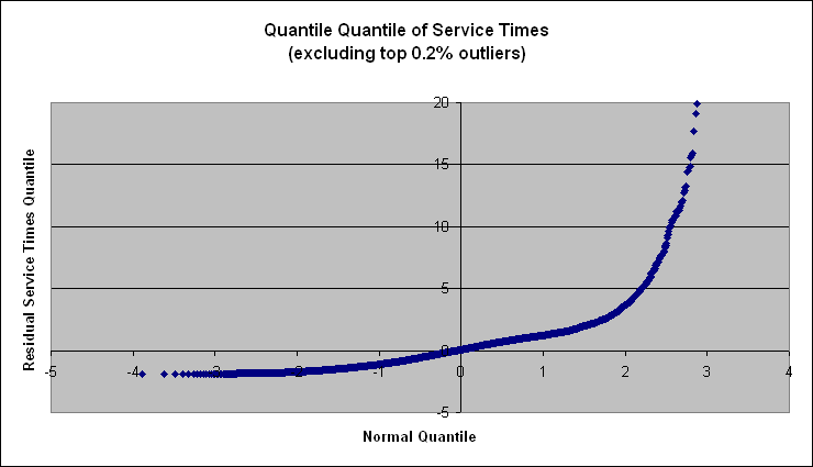
Figure 4: Q-Q Plot of B[1] Service Times (excluding 10 outliers)
The analysis of inter-arrivals and service times being done at a single point in the queuing network. To rigorously test the model assumptions, the distribution of inter-arrival times as well as service times at every computational and inter-connect resource should tested. To make this possible, future work should include a comprehensive statistical test for every node. A graphical test is still a good way for the user to convince themselves that the assumptions underlying the model are relatively safe.
5.2 Model Verification Results
For the example application, walk-throughs were done to verify that data moved through the simulation modules as expected for a few test cases. A rudimentary sanity check was done by confirming that block output times occurred chronologically after block input times. It is hard to quantify program correctness, and a technique that can help in verification is an animation . A tool that shows the movement of data through the queue network model is currently under construction. Once it is completed, it can help the programmer quickly locate suspicious behavior which might indicate the presence of programming errors.
5.3 Operational Validation Results
To validate the simulation results against operational results, the
application was run 5 times. The means from these runs is given in the
following table:
| Service Times | System Runs (�s) | Simulation Runs (�s) | ||
| Run | Mean | Standard Deviation | Mean | Standard Deviation |
| 1 | 3036.68 | unknown | 3037.31 | 479.35 |
| 2 | 3255.19 | unknown | 3255.89 | 3014.38 |
| 3 | 3137.57 | unknown | 3138.10 | 7659.73 |
| 4 | 3030.52 | unknown | 3031.22 | 413.61 |
| 5 | 3110.39 | unknown | 3114.02 | 1885.79 |
| overall mean | 3114.07 | 3115.30 | ||
| overall std dev. | 91.45 | 91.42 | ||
Table 1: Results Summary from System and Simulation Runs
There are many important points to note here. Let us examine the system
run means first. The five runs generated an overall mean of 3114.07�s with
a standard deviation of 91.45�s. Using a t-table distribution with n=5, we
get a confidence interval of 3114.07�s?84.27�s at 95% confidence, which is a
narrow band showing relatively high confidence for the execution time. The
variability here is very low, and can be reduced even further by simply doing
more than five runs. Another measure of variation is the coefficient of
variation (COV). The COV is calculated as the ratio of the standard
deviation to the mean, and in this case it is only 0.029. All the standard
deviations for the system runs are listed as "unknown". This is because,
as mentioned previously, real system runs do not allow a comprehensive trace to
be generated. Only the means are recorded because they require a simple
running sum to be updated during actual execution, and thus have a minimal
effect on the running time.
Let us now move our focus to the simulation run results. Comparing the means for the individual simulation and system runs, it is very clear right away that there is a high correlation between the simulated and actual results. Statistically, the correlation between the two is calculated to using the formula given below. The correlation for our data is extremely high, calculated to be 0.99989. This is a very important value that can be automatically calculated using the equation and can give a single figure to show the operational validity of the simulation
.

Figure 5: System (x) and Simulation (y) Correlation Equation
Finally, let us examine the standard deviations for the simulation runs.
The standard deviations for runs 2, 3 and 5 are very high, with COV ratios of
0.93, 2.44, and 0.61. These high COV values suggest that characterizing
the block performance simply using a mean and standard deviation will not
provide a very accurate model. Examining the individual service
times provided by X-Sim show that there are a few outliers that are skewing the
distribution away from the model. These might represent times when unusual
events like context switches or heavy disk accesses occurred. Excluding
the top 5% gives the following revised data:
| Service Times | System Runs (�s) | Simulation Runs (�s) | ||
| Run | Mean | Standard Deviation | Mean | Standard Deviation |
| 1 | 3036.68 | unknown | 2991.67 | 201.41 |
| 2 | 3255.19 | unknown | 3017.09 | 208.41 |
| 3 | 3137.57 | unknown | 3001.13 | 209.53 |
| 4 | 3030.52 | unknown | 2970.57 | 198.45 |
| 5 | 3110.39 | unknown | 2984.16 | 199.61 |
| overall mean | 3114.07 | 2992.92 | ||
| overall std dev. | 91.45 | 17.53 | ||
Table 2: Results When Top 5% Outliers are excluded
Now the standard deviations are much lower and give us much more acceptable COVs. Shown below is the Q-Q plot for the service times when the 5% top outliers are excluded.
.
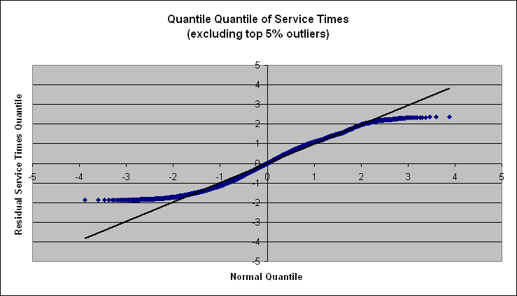
Figure 5: Q-Q Plot of B[1] Service Times (excluding 5% outliers)
This plot displays normal like behavior but with short tails. This matches what one would expect. As discussed before, B[1] iterates n times where n is a uniformly distributed variable. The Q-Q plot above shows a uniform distribution with normally distributed noise.
5.4 Summary
The behavior of block B[1] can be summarized from the above analysis. Excluding 5% outliers, block B[1] runs with normally distributed service times which can be represented by a simple confidence interval of 2992.92�s?5.32�s at 95% confidence. However, the top 5% outliers represent an important factor because they take a lot longer to execute, and they represent disruptive operations like context switching and disk accesses. One solution is to migrate to a more dedicated platform where those disruptive factor do not cause much of a problem. That would allow the block to simply be represented by an execution time of roughly 3ms?.04ms.
6 Summary
X-Sim is a simulator that has built to be used with the Auto-Pipe system. It allows users to simulate their applications on a given set of heterogeneous resources before deployment, allowing both correctness testing and performance analysis. The comprehensive gathering of trace data provides opportunities for the user to analyze and better understand their application's behavior. However, for X-Sim to be trusted by potential, it requires rigorous verification and validation. Graphical displays help show the user that key assumptions are maintained. Statistical properties of the model, system, and simulation can be related to each other to be able to give confidence intervals of performance estimates. Unfortunately, the current measurement techniques in the system and simulation are slightly different so comparing them is sometimes misleading, as seen in this case when the application being studied has very small service times that are prone to be overshadowed by overhead. Future studies on X-Sim should be done when more consistent measurement techniques have been implemented, and an application that consists of blocks that take substantial time should be studied. The end goal is to allow general simulation validation for any application, and generate sufficiently confident performance estimates. This would allow users to create mappings that perform faster not only in simulations, but reliably in the real world too.
References:
[ Gayen06] Gayen et. al., "X-Sim: A Federated Heterogeneous Simulation Environment",In Proceedings of 10th High Performance Embedded Computing (HPEC) Workshop, September 2006, pp. 75-76
Available at: http://sbs.cse.wustl.edu/pubs/gtfcc06.pdf
[
Tyson06] Tyson, "Auto-Pipe and the X Language: A Toolset and Language for
the Simulation, Analysis, and Synthesis of Heterogeneous Pipelined
Architectures",
Master's Thesis, Washington University Dept. of Computer Science and
Engineering, August 2006.
[ Tyson05] Tyson, "X Language Specification 1.0",
Washington University Dept. of Computer Science and Engineering Technical Report
WUCSE-2005-47
[ Sargent04] Sargent, "Validation and
Verification of Simulation Models",
This paper appears in:
Simulation Conference, 2004.
Proceedings of the 2004 Winter
[ Balci95] Balci, "Principles and techniques
of simulation validation, verification, and testing",
Proceedings of the 27th conference on Winter simulation - Volume 00, 1995
[ Kleijnen95] Kleijnen, "Statistical
validation of simulation models",
European Journal of Operational Research 87, 1995, pp.21-34
Acronyms:
COV
Coefficient of Variation
DSP
Digital Signal Processor
FPGA Field
Programmable Gate Array
GNU GNU's Not
Unix
GPP
General Purpose Processor
GPU
Graphical Processor Units
HDL
Hardware Description Language
Q-Q
Quantile-Quantile
This report is available on-line at http://www.cse.wustl.edu/~jain/cse567-06/xsim.htm
List of other reports in this series
Back to Raj Jain's home page